Evaluating forecast accuracy is an essential part of demand planning and inventory optimization. In practice, it is considered one of the key indicators that companies rely on. In our experience, however, it's importance is overstated and businesses often have a mistaken view of its impact on their bottom lines. In this article, we will discuss five key problems that may arise when using forecasting accuracy, and offer up a few solutions.
Let's start with why we would want to calculate demand forecast accuray in the first place. We might need it for several reasons:
- To choose the optimal forecasting model
- To calculate safety stock
- To identify SKUs that need special attention
- To compare different software products
Forecast accuracy can be calculated using forecast error. The error in this case is the difference between the actual value of demand and its forecast value. In other words, the greater the forecast error, the less accurate the forecast. For example, with a forecast error of 5%, the forecast will be 95% accurate. But the biggest pitfall, as we will see later, lies in the multitude of methods used to estimate the forecast error.
98,1%
What might be hidden behind these figures? An infinite number of metrics calculated in completely different ways, such as:
 The results can vary significantly from case to case. Let’s formulate the first problem of using the forecast accuracy as the main criterion for evaluating inventory management KPIs.
Problem 1. Forecast errors can be calculated using different metrics, which give very different results that can't be compared against one another.
To better illustrate this problem, consider the following example:
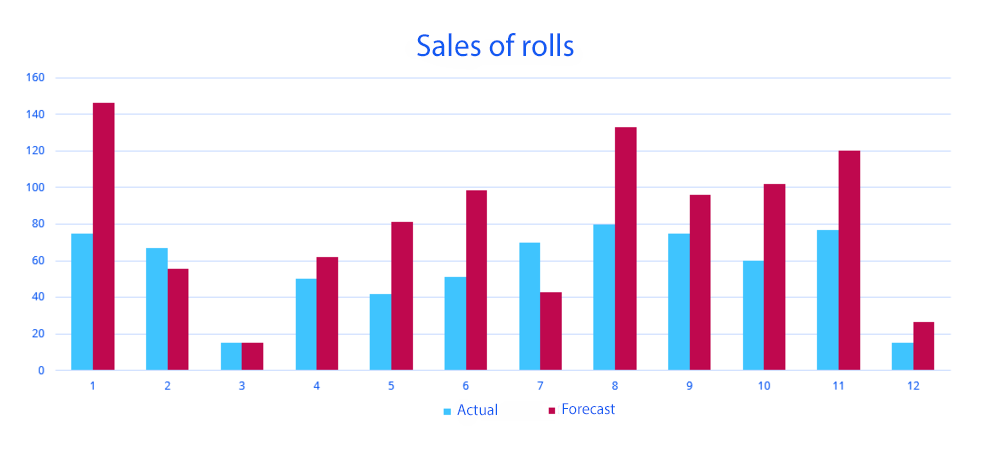 The graph shows sales of rolls over the last 12 days, and below is the forecast error calculated using various techniques.
| Forecast error | |
| MAD | 31.610 |
| MSE | 1.407 |
| RMSE | 37.5 |
| MAPE | 55% |
| sMAPE1 | 23% |
| sMAPE2 | 42% |
As you can see, the forecast accuracy number we get varies greatly. You can manipulate these statistics to your liking. Some employees may choose a specific metric and provide management with the expected results. Or they might close a project with numbers that will present it in a positive way. In some cases, companies may even deceive themselves without realizing it, assuming better performance than is actually the case.
Solution 1 Establish a specific metric for evaluating the forecast accuracy and a calculation technique at the company level
Problem 2. How to evaluate the forecast accuracy for a product group and for business overall
Now we need to somehow scale up this metric across the entire company. Let’s say we have 100,000 SKUs whose sales can vary dramatically. They cannot simply be averaged. For example, we have two products, whiskey, and sausage, with the following numbers:
| PRODUCT | FORECAST | ACTUAL | MAD | MAPE |
| Sausage | 100 | 50 | 50 | 50% |
| Whiskey | 50 | 100 | 50 | 100% |
| ... | ... | ... | ... | ... |
| Total | 150 | 150 | 0 | 0% |
If we add up the forecast and actual sales for these products, they will balance each other out. The forecast accuracy will be 100%. However, if we look at the numbers separately for each product, things don't look quite as good.
Moreover, if you look closer you’ll see that the deviation of the actual value from the forecast is the same for both products, but the MAPE is 50% in one case and 100% in another. You might have already guessed this is due to the fact that the actual sales deviate in different directions. This is another problem with this approach, which we will come back to in a bit.
To solve this problem, we can choose to weight these errors according to their contribution to significant criteria for the business. We might choose profit or sales volume.
For example, we weigh whiskey and matches by average demand. In this case, the error shifts to the product that sells more. As a result, we get a more or less correct estimate of the forecast accuracy.
| PRODUCT | AVERAGE DEMAND | MAPE %1 | wMAPE 1 | MAPE % 2 | wMAPE 2 | MAPE % 3 | wMAPE 3 |
| Whiskey | 100 | 50% | 10% | 90% | |||
| Matches | 1000000 | 50% | 90% | 10% | |||
| ... | ... | ... | ... | ... | ... | ... | ... |
| Total | 50% | 89,99% | 10,01% |
Solution 2 Use errors weighted by business KPIs to evaluate the forecast accuracy
Now let’s take a look at high and low forecast accuracy levels from a different perspective
Problem 3. High and low forecast accuracy levels are not a key driver of economic performance
For many SKUs, high or low forecast accuracy is not a key performance driver. Do not treat these mathematical errors as something that should always be used to evaluate the quality of inventory management. We need to keep in mind that these methods come from the field of pure mathematics and were intended specifically for statistical and mathematical - not business performance - indicators.
For example, MAPE was initially used to forecast normally distributed time series, such as electricity consumption. Only later was it applied to demand forecast accuracy. Yet, when it comes to sales, only about 6% of items actually show a normal distribution. Usually we're talking about daily grocery and food items.
Let’s consider slow-moving goods, such as household chemicals that consumers tend not to need every day.
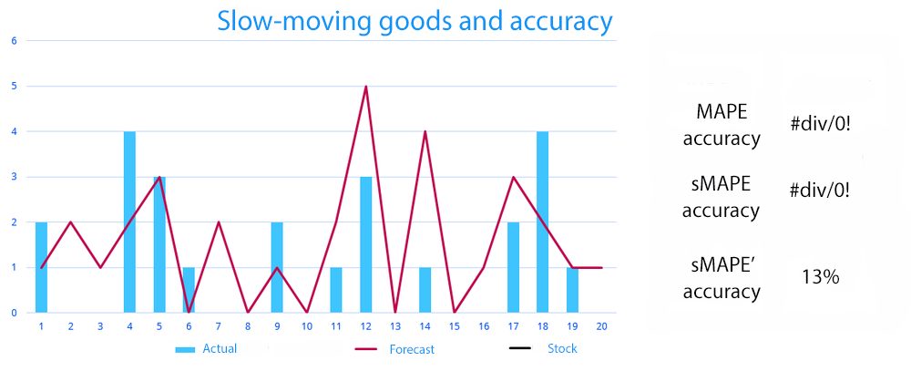 As you can see from the graph, many metrics simply do not work here. MAPE and sMAPE accuracy cannot be calculated. Even if we manage to somehow “align” the data, we will get a dramatically low accuracy – 13%.
Now let’s look at the subject area, not just mathematical errors:
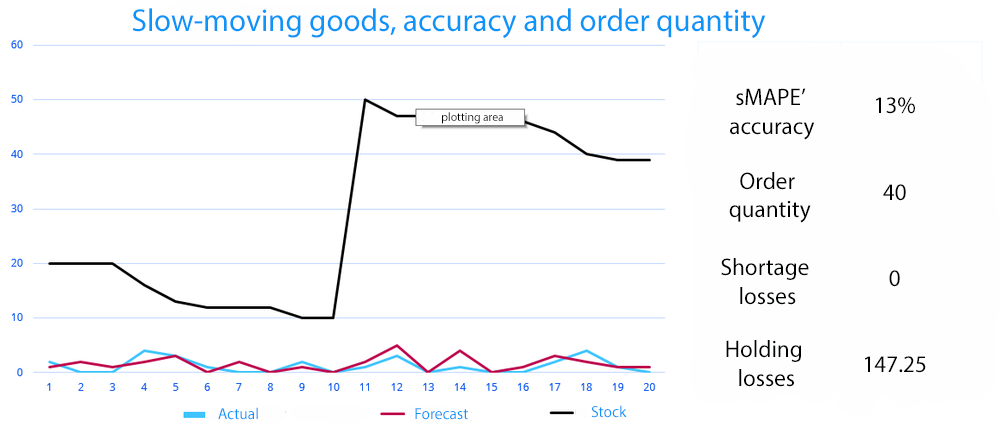 Here we can see that the forecast accuracy does not affect anything at all, because the stock depends on the minimum order quantity or delivery frequency that the supplier can provide. As a consequence, this figure is of little practical value for us. Of more concern would be negotiations with suppliers, rather than increasing the forecast accuracy.
Past shortages and high forecast accuracy
On the other hand, past shortages may also lead to inaccurate forecasting. They lead to lower sales, meaning that the accuracy can be overestimated or underestimated.
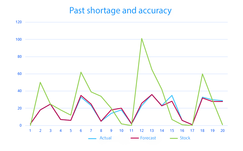 In the example, the MAPE accuracy is 95%. Shortages are a common occurrence, and our forecasts tend to underestimate demand during those times.
Solution 3 Evaluate the forecast accuracy for target inventory levels rather than relying solely on mathematical errors
Problem 4. MAD, MSE, RMSE, and MAPE are mathematical errors. They tell us nothing about profits.
From what we’ve seen in the industry, the mean average percent error (MAPE) and variations of it are the most common method used to estimate forecast error. The mean absolute error (MAE), the root mean squared error (RMSE), and the mean absolute deviation (MAD) are also common.
Despite the fact that most companies still use the above methods, we believe their lack of precision makes them less than optimal for use in real business situations.
These approaches are more related to mathematics than to business. They provide us with basic numbers that tell us nothing about real money. Real decisions are based on the financial benefits they can provide. For example, an error of 80% at first glance sounds intimidating. But in reality, it can reflect a number of different situations going on in our business. An error involving nails that cost 50 cents per nail unequivocally means losses. But not the sort of losses we’re looking at from the sale of industrial equipment worth 700,000 dollars at that same level of forecast error. Nor can we forget about volumes, something also ignored by these errors.
Another key issue is the money that ends up tied up in inventory and lost profits from stock-outs. For example, if we predict the sale of 20 rims, but actually only sold 15, the cost of our error is 5 rims, which we will have to pay holding costs for over a specific period of time, and therefore the cost of tied-up capital at a certain percentage. If we consider the opposite situation, however, we forecast the sale of 20 rims and get orders for 25. Now we're dealing with lost profits, or the difference between how much we ordered and how much we actually sold. We have the same forecast error in both cases, but the results can differ dramatically.
Let’s look at an example with spoilage.
 We see fairly good forecast accuracy – 85.95%. The black bars represent the quantity of product that we over-forecasted and had to write off. The total loss of the company is 2,270 dollars.
The total loss of the company is 2,270 dollars. This time, sales are consistently underestimated.
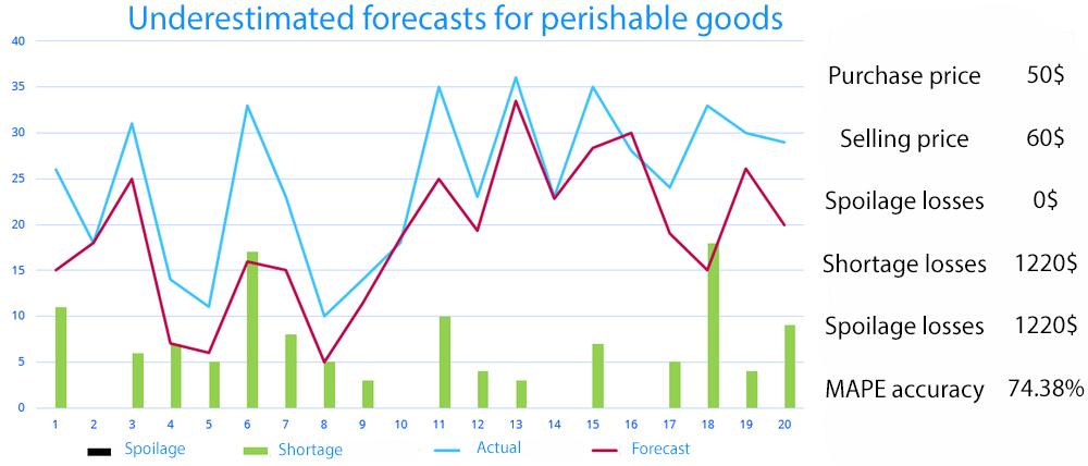 The forecast accuracy here is much lower – 74.38%. We should have chosen the first forecast because its accuracy is significantly higher. But in the second case, the total loss of the company decreased by almost half – up to 1,220 dollars. With this purchase price, selling price, and demand dynamics, it is more profitable for the company to underestimate demand than to overestimate it.
This shows that a percentage-based metric may not always reflect actual business performance. Therefore, we can calculate two different values. If the forecast turns out to be less than the actual demand, it will lead to a stockout, the loss from which can be calculated by the formula:
Loss = quantity of unsold products* (selling price – purchase price)
For example, say we buy rims at 3,000 dollars a piece and sell them for 4,000 dollars a piece. Our first month's forecast was 1,000 rims sold, but we received orders for 1200. In this case:
Loss = (1,200–1,000)*(4,000–3,000) = 200,000 dollars.
If the forecast exceeds actual demand, the company will incur losses from holding costs. In this case, the loss can be calculated as follows:
Loss = cost for unsold products * rate of return (ROR) on alternative investments
Let's suppose that actual demand in the previous example was 800 rims and we had to hold the rims for another month. Let the rate for alternatice investments be 20% per year. Then:
Loss = (1,000–800)*3,000*0.2/12 = 10,000 dollars.
And so we will consider one of these values in each specific case.
Solution 4 Calculate the forecast error in monetary terms
Problem 5. Only the accuracy of real-time forecast is evaluated. However, safety stock can reach 70% of the total stock
The errors considered above apply only to demand forecast and do not describe the safety stock. In some cases, the safety stock can be 20–70% of the total inventory on hand. Therefore, no matter how accurate the forecast is from the perspective of the methods described above, they igore safety stock. This means that real data may be significantly distorted. Therefore, even with a highly accurate forecast, the company may suffer large losses and underperform.
The safety stock can be calculated in different ways:
- Intuitively by company employees
- Percentage of average daily sales
- Normal distribution for demand, forecast errors or lead time at a fixed cycle service level
To solve this problem, we suggest comparing algorithms using the concept of service level. The service level (which we will refer to as Type II service level or fill rate) is the amount of demand that we can meet using inventory on hand during a replenishment cycle.
For example, a 90% service level means that we will be able to service 90% of demand. While at first glance, it may seem logical that the service level should always be 100% to maximize profits, this is not the case in reality: meeting 100% of demand means extreme over-stock, and - in the case of perishables and fixed shelf life products - spoilage and waste. Not to mention that holding costs, spoilage, and capital costs will ultimately reduce profits over what could be earned at a service level of 95%. It should be noted that each individual item will have its own target service level.
Since the safety stock can account for a lot of what we're looking at, it cannot be ignored when comparing algorithms (as is the case when we calculate errors using MAPE, RMSE, etc.). Therefore, we do not compare the forecast, but target stock for a fixed service level. The optimal, target stock for a fixed service level is the amount of goods that must be kept in stock in order to achieve maximum sales profits while minimizing holding costs.
As the main criterion for the quality of forecasting, we will use the total value of losses for the service level described above. Thus, we estimate the losses in monetary terms when using this particular algorithm. The smaller the loss, the more accurate the algorithm.
We should note here that the optimal target stocking level can also differ for varying service levels. In some cases, the forecast will be right on target, while in other cases it may be skewed in either direction. Since many companies do not calculate a target service level, but use a fixed level, we calculate the main criterion for all the most common service levels: 70%, 75%, 80%, 85%, 90%, 95%, 98%, 99% and then sum up the losses. This allows us to test how well the model works overall.
Let’s look at an example with several methods. For each of them, we can evaluate what stock it suggests at different service levels. Using historical data for the past six months, we can calculate what this would lead to: how much actual demand would be satisfied, how much stock would be on hand, how many units would have to be written off, etc. We can represent all these total losses in one figure.
| Losses in dollars | Method 1 | Method 2 | Method 3 | Method 4 |
| Total value for common service levels (80%, 85%, 90%, 95%, etc.) | 965,314 | 947,936 | 866,907 | 1,290,989 |
In this example, method No. 4 will be the least effective, while method No. 2 will be the most effective.
Solution 5 Plan product stocks according to a fixed fill rate
How can the model be further improved?
Using a fixed service level is now an obsolete method. Modern software makes it possble to dynamically manage the service level for each item. You don’t need to do this yourself or consult an expert. The program itself will determine what is more profitable: keeping a few dozen extra units in stock or, on the contrary, running into a stock-out situation. The service level for a specific SKU will be calculated automatically, taking into account all possible risks. This is called the target service level.
This approach forces us to consider the forecast error in a completely different way. In this case, the loss is basically the ratio of losses at the target service level in terms of the expected (according to the model) vs actual (observed) distribution of sales.
The predicted target service level does not always correspond to the actual optimal level already in use. Therefore, we need to compare the error between the forecast sales at the target (according to the model) service level and the actual sales volume that provides this service level according to company data.
Let’s use the previous example of rims to illustrate this point. Suppose that the predicted service level is 90%, and the optimal stocking level for this case is assumed to be 3,000 rims. If we assume in the first case that the actual service level was higher than the forecast at 92%, then volume of orders also increased to 3,300 rims. The forecast error is found from the difference between the real and actual sales volume, multiplied by the difference in selling prices. To sum, we have:
(3,300–3,000)*(4,000–3,000) = 300,000 dollars.
Now, let's consider the opposite situation: the actual service level was 87%, less than predicted. Actual sales came in at 2,850 rims. The forecasting error is found by adding the cost of unsold inventory multiplied by the ROR for alternative investments in the same period (for our example we look at one month and use a ROR of 20% annually). The total value of the criterion will be equal to:
(3,000–2,850)*3,000*0.2/12 = 7,500 dollars
The criteria we use, in contrast to classical mathematical errors, show the total losses in money terms when comparing various models. Since the target service level can change, we combine the approaches – the calculation of losses at the target service level and the total losses at common service levels. And so the best model will be the one that minimizes losses. This approach will allow businesses to evaluate the operation of various algorithms in a language they understand.
Example of comparing four methods using two criteria. The lower the losses, the more efficient the method.
| Losses ($) | Method 1 | Method 2 | Method 3 | Method 4 |
| Losses at the target service level | 1,724,804 | 1,076,983 | 1,597,437 | 1,954,575 |
| Total losses at common service levels | 965 314 | 947,936 | 866,907 | 1,290,989 |