What is a digital twin?
In recent years, there has been a lot of talk about digital twin technology. Generally, a digital twin is a virtual copy of a process or physical object. Digital twin technology includes a set of mathematical models that constantly receive data from the real-life environment. Based on the collected data, a digital twin is built and changed.
This technology is used to test hypotheses. It allows you to save money and choose the best solution. Let's assume that you are planning to expand the range of products in your store. Simulating the situation in a virtual environment helps to see how often deliveries are to be made, whether there will be delays due to higher volumes, whether your acceptance team will handle the load, whether cannibalization will happen if new brand lines are introduced, etc. In this way, all bottlenecks can be identified beforehand.
In inventory management, a digital twin can be used to handle the following tasks:
- Defining an optimal stocking level;
- Plan transfers from suppliers, and between warehouses and points of sale;
- Simulating the distribution of stocks through the distribution center;
- Simulate stocking levels during promotions;
- Identify potential for stock-outs, repacking, and short and partial shipments;
- Reviewing possible scenarios.
At Forecast NOW!, we use digital twin technology to forecast and calculate the optimal stocking level. This is a complex and time-consuming process that involves many factors.
Business is all about risk management in a constantly changing environment. To maximize performance and profit, you have to be able to quickly respond to changes. Yet in practice, analyzing all possible scenarios in a real-life environment is impractical, especially when inputs change every day. This is the reality faced by most merchants.
To optimize a company's inventory level in terms of profit, Forecast NOW! builds a digital copy of the company's inventory management processes. It then simulates possible scenarios, usually running around 100,000 experiments. The model output shows how likely it is that a particular quantity of stock will be sold out, giving insights on how much product quantity should be ordered that day (or on another day) to maximize profit, maintain the desired service level, or make decisions based on other objectives.
How it works in practice
Before delving into the details, let’s consider a simple example of how technology can model a coin toss.
Let's assume that we have an ordinary coin. No coin is perfect - i.e., it's not likely that 100 tosses will result in 50 heads and 50 tails. Most likely, you will get 60/40, 48/42, or some other similar split.
If we want to obtain statistically reliable data, we need to toss the coin many times – 100,000, let's say. Clearly, this would be incredibly time-consuming.
Instead of running through this manually, we can digitize the coin as accurately as possible. We will reproduce all its chips, pocks, bumps, and pits. We will take into account all the laws of physics and all the forces acting on the coin. The result is a digital twin of the coin which is as identical as possible to the actual coin.
Now let’s toss the digital twin of the coin 100,000 times. Let's sya we end up with 55,000 heads and 45,000 tails. This suggests that in real life, we would expect a 55% chance of getting tails.
What should we do with these probabilities? An example with a weather forecast may help us here. If forecasters say there is an 80% chance of clouds and a 20% chance of rain today, you know there is a risk of getting wet, albeit a small one.
They could ignore that probability, average out, and just say, "It will be cloudy today." If you are planning a long walk, it would be unpleasant to get wet. So if you know there is a small chance of rain today, you can play it safe and take an umbrella. On the other hand, if you plan to spend the day in a car, the rain is not terrible, and you won’t need an umbrella at all.
Either way, it is better to be aware of the chance of rain and able to decide whether you need an umbrella.
If we apply this analogy to inventory management, we get a comparison between probabilistic and classical models. Classical methods include average daily sales, moving average, ARIMA, Holt-Winters' method, and other more complex algorithms. These methods are usually implemented as a 1C module or Excel spreadsheets. All of them have a single output number, like a demand forecast. That's what we focus on. According to average daily sales, if we sold 5 units yesterday and 10 units today, the forecast for tomorrow is 7.5 units. In reality, it could be more or less than that.
Returning to the comparison, say, for example, that the algorithm shows that next week's demand will be 25 Snickers. We don't have any other data other than that. What if you knew that with a 30% chance, you could sell 50 Snickers next week and earn twice as much? And, let's say, you have the funds to make the purchase and the space in your warehouse.
Estimated demand is only one of the quantities that can be calculated probabilistically. For example, when you put in an order to a supplier, you can't be sure that it will be delivered on time. If you know that the risk of lead time delay is 40%, you have a chance to think about whether to order the quantity you've planned or increase it to avoid a stockout in the future.
Knowing the probability of all possible scenarios enables you to manage your stock more flexibly and efficiently.
Let's get back to the digital twin technology and exactly how it works in Forecast NOW!
The algorithm takes sales and inventory history for past periods.
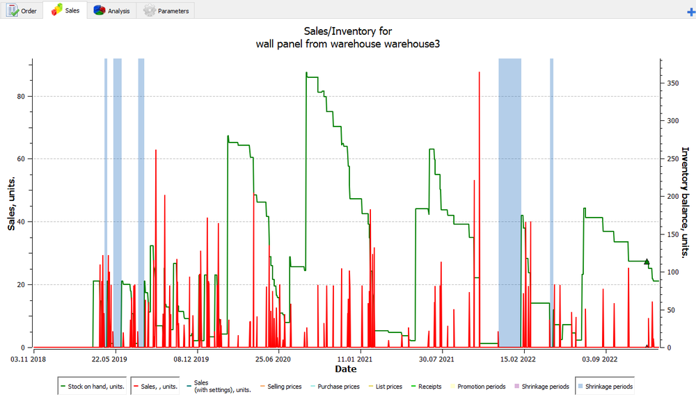
Fig. Sales and Inventory History for Past 4 Years.
The history usually includes periods of shortage, abnormal surges in sales, seasonal demand fluctuations, promotions, etc. The software clears sales from all these periods, turning the data into a demand history.
After the history is cleared, the software creates a digital twin of your product. All possible characteristics of product demand are collected. For example:
- How often the product was sold every day;
- How often the product was sold every other day;
- How often the product was sold every two, three, four, or more days;
- How often one unit was sold today, two units – tomorrow, three units – every other day, etc.;
- How often two units were sold today, two units – tomorrow, three units – every other day, etc.;
- Other options.
In other words, all possible frequencies of sales volumes in a past period are determined for each product on a specific date of order. If new sales data for the previous day appear, the digital twin will be rebuilt and all models will be recalculated using the new data.
As soon as the digital twin of a particular product is ready, we can simulate possible scenarios for future events, i.e. how demand for the product will change. For this purpose, the software runs 100,000 experiments in the virtual environment.
Let's consider a simulation case.
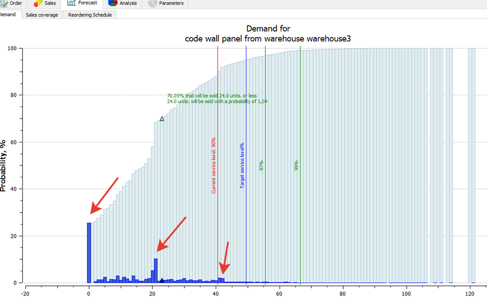
Below, the horizontal axis shows possible demand volumes, and the height of dark blue columns represents the probability we will see that level of demand. To put it another way, this is the number of experiments in which exactly a given quantity will be sold:
- Column No. 1 shows that no unit was sold in 13,000 experiments. This means that there is a 16% chance that no unit will be sold.
- Column No. 2 shows that 21 units were sold in 5,000 experiments. This means that there is a 5% chance that exactly 21 units will be sold.
- Column No. 3 shows that exactly 42 units are sold in 900 experiments. Accordingly, the probability of such sales is less than 1%.
- And so on...
This model provides the sales probability distribution without averaging any values.
And now what?
Our task is to cover a certain number of possible scenarios. For example, the target level of service is 90%. In the figure above, it is represented by the red line. The corresponding demand volume is 41 units. To the left of this line, all dark blue columns represent 90% of all possible scenarios, i.e. the demand varied from 0 to 41 units in 90,000 digital experiments.
This means that we should have 41 units in stock in the warehouse to meet a 90% service level. If you need a 99% service level (the green line in the figure), you should have 67 units available in the warehouse.
This case shows a digital twin for a single product. In real-life settings, an individual digital twin is built for each product with its unique features. Then the software simulates possible scenarios for each specific product.
Obviously, it's not possible to test so many hypotheses in a real-life environment. Therefore, classical methods (average sales, Arima, Holt-Winters' method, etc.) average the final demand values and often compromise on the quality and accuracy of forecasts. Conversely, when building a digital product model, we deal with each SKU individually and consider all possible demand scenarios for them.