- Part I. Why you should not predict sales for inventory management?
- Part II. Can you should you - always forecast demand?
- Scientific background
- References
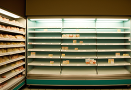
Most companies use demand forecasting methods that are 10-15 years behind: exponential smoothing, ARIMA, moving averages, the Holt-Winters method and others. They are not only out of date, but also ineffective in solving the problem of inventory management for 94% of product mixes in the food and beverage industry, and for almost all non-food items, as countless research has demonstrated (see the scientific background). As a result, businesses waste 20 to 40% of working capital on overstock and can lose up to 5-10% of revenues due to stock-outs. These methods all ultimately forecast a single number in the end, which is often akin to reading the tea leaves. Safety stock is added either “by eye” or according to standard distributions of demand, which simply do not correspond to these goods. Now we have access to vast computing resources that make new 4th generation forecasting technologies accessible.
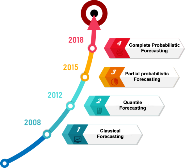
Fig 1. The development of forecasting algorithms.
For 4th generation algorithms to be effective, they must use historical data and be understood by employees. Historical sales statistics do not reflect the basic dynamics of demand and needed to be purged and cleansed of low demand periods, promotion-based peaks, one-time large sales, etc. Comparisons of the accuracy of such methods also differs and is expressed in terms of losing sales, and not MAPE or RMSE errors, which are essentially meaningless to business. This requires managers and front-line employees alike to change their thinking.
In the first part of our guide, we will cover the following issues:
- Why do we need to process sales data before building a forecast?
- How do we prepare sales data?
- How does this influence the end result?
If you are already an experienced specialist, you can skip straight to the second part of the manual. In it we cover:
- Why should we forecast inventory and stocks, and not demand?
- What are the advantages of probabilistic forecasting methods?
Probabilistic algorithms are considered the most advanced method for managing inventory. Using 4th generation probabilistic forecasting methods, we can predict the entire product mix up to Group Z, and not only calculate the optimal stock for each store and warehouse based on exact reorder dates, but also account for changes in lead times and the effects of advertising and promotions. Moreover, these algorithms can themselves suggest the optimal service level for each unit in each order. This also helps businesses achieve a balance between stock-outs, holding costs, opportunity costs, spoilage, and other factors.
Part I. Why you should not predict sales for inventory management?
Often, in order to determine the necessary inventory, we first build a sales forecast based on historical data and then calculate the safety stock. All seems good - in the end we have our required stock that we need to meet demand at our particular desired service level.
However, when predicting sales we're using historical data which often is not an accurate reflection of current demand. We need to instead forecast demand. But where do we find the demand history, if we only recorded sales? And what are the main differences between these apparently similar terms? In this part of the guide, we would like to share our experience in teasing out demand from sales history. We will look at stock-outs, anomalies, marketing promotions, slowing moving goods, and pseudo-kits, as well as how to manage inventory up to 99% of the entire product range, and not just the AX group.
Past Stock-Outs - Dangerous in the Future and the Past!
The first important nuance here is shortages or stock-outs in the past. For example, last month we had days when items were not on the shelves, sales were zero. What would happen if we made an according to the simplest model of demand forecasting - the average? Suppose sales in other months were 600, 500, 600, and in the month when there was slow demand or stock-outs, fell to 300. We get the forecast for the simplest model: (600 + 500 + 600 + 200) / 4 = 475. Obviously, 475 units will not be enough for us for any of the months with normal demand.
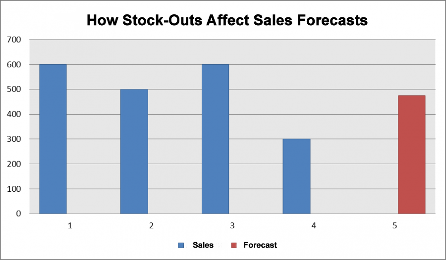
Fig 2. How Stock-Outs Affect Sales Forecasts.
What will happen if we order 475 units? We will only be able to sell 475 regardless of demand. Demand, as we know, was much higher in other months. So we'll lower our next order to 468 units. We will fall into a vicious circle of deficit and artificially limit demand. So, how to solve the stock-out problem?
First step
The easiest way to solve this problem is to flag days where there were stock-outs, and we simply could not sell anything - we'll refer to them as OOS days. In our example, 01.12., 01.19, and 01.20.
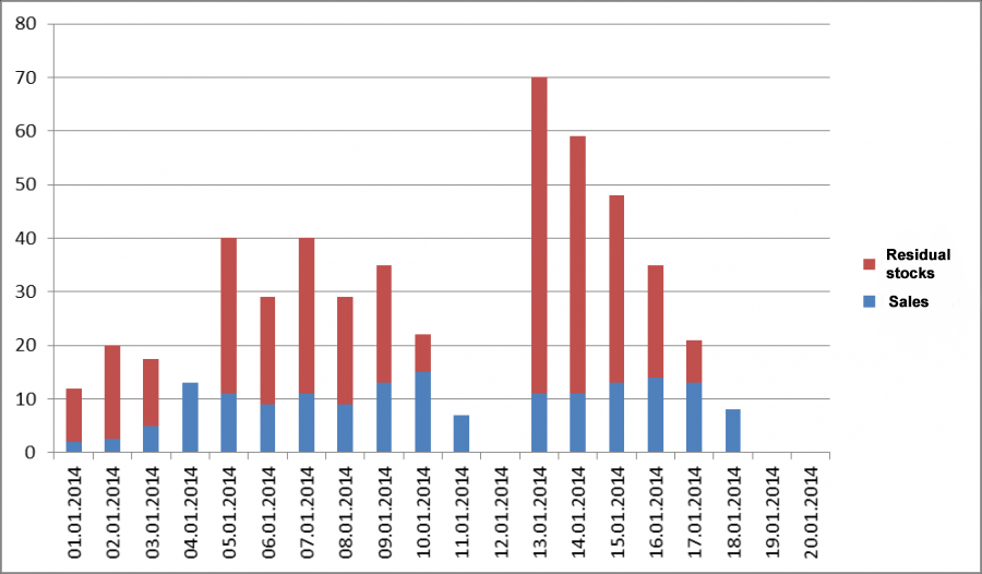
Fig 3. We flag days with zero inventory as OOS days.
Average sales before history cleansing = 8.49 units Average after completing the first step - 9.85
Step Two
For the next step, we flag any days (periods) in the sales history where inventory dropped below the average daily sales volume for a given item as OOS days (periods). This could be caused by shrinkage and similar events.
Average daily sales are calculated from the data we obtained after the first step (i.e., they don't contain any information on zero sales on days where there were stock-outs).
It's also a good idea to clean the historical data of any unusually high peaks in sales which could distort our average. For example, in January, one customer bought 12 thousand bolts, while average sales per month are 1 thousand units. So, the average for one year will be 2 thousand units, and we will mark all sales as unreliable. The median can also be used instead of the average. The median is more resistant to spikes in demand.
Pro Tip: before calculating the average, remove spikes in sales or use the median.
In our example, the mean sales for all days excluding 01.12, 01.19, and 01.20 is 9.85 units. The median is 11 units.
|
2 |
4 |
5 |
7 |
8 |
9 |
9 |
11 |
11 |
11 |
11 |
13 |
13 |
13 |
13 |
14 |
15 |
We'll use the median and flag all periods where inventories were lower than the median level (11) as OOS days. The diagram below shows the data after omitting stock-outs and and potential OOS periods.
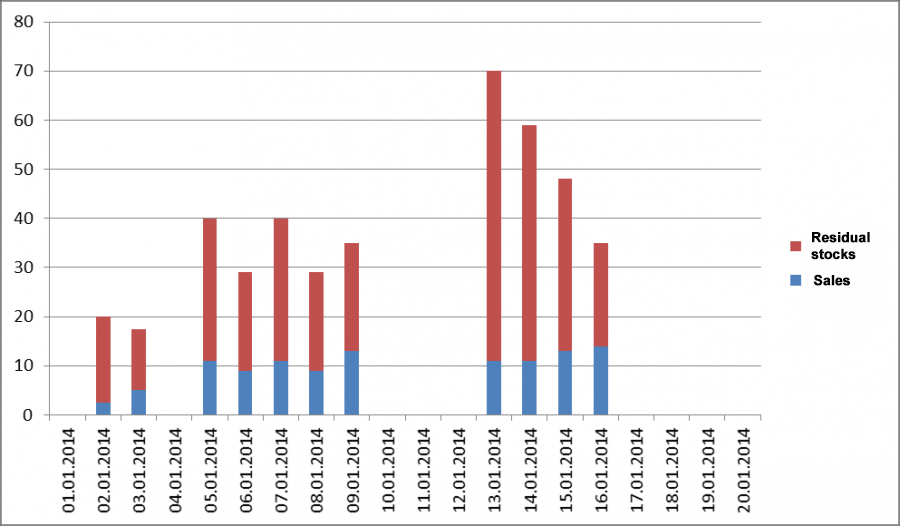
Fig 4. We flag days with inventories lower than the median as out-of-stock days.
Average sales are now 9.95 units. It is easy to see that the difference is almost 1.5 units, or 17% of the total demand!
Step Three
There are additional complexities and nuances which we need to be aware of some times. For example, kits and sets. If you have 3 candles in stock but customers usually buy 4, you have a potential OOS , although this may not be recognized after the first two steps.

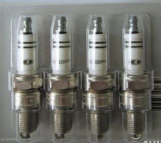
Fig 5. Candle Sets
That's why in the third step, we determine such kits or sets, which may also consist of different units, and flag all days where inventories drop below the necessary minimum as OOS days. In our example, for candles it will be 4 units.
Tip: think what kits or product sets you may have in your business and track them.
Now we have sales history data where potential stock-outs and understocked kit pieces have been flagged. It is worth noting that distortions in the sales history can also occur due to the fact that goods are simply not put on the shelf, although they are in stock in the warehouse, or due to resorting. All these factors should be borne in mind, and if they are something that happens in your business, you'll need to find a way to omit them from your sales history data.
Step Four
What should we do with the stock-outs we've found? As we've already learned, if we simply ignore stock-outs, we can easily fall into a vicious circle and end up permanently understocked.
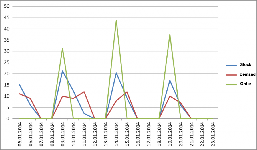
Fig 6. Sales history with stock-outs omitted.
There are several options.
First, we can simply ignore these periods, delete them from the sales history and forget about them. There is something to be said for this approach. But what about the drawbacks?
Imagine that you are selling a product that was only in stock 5% of the time, and that it sold in large numbers every day. Is this then the demand profile for this product? Is this the sales velocity we would see, and if we had it in stock all the time we would sell 20 times more units? Most likely the answer is no. Especially if we're offering consumers a unique product.
Demand doesn't have a chance become saturated, buyers are quickly snapping up what's in stock. What would happen if we used this metric? We would order much more inventory than we really need. What can we do about it? Ditch this approach if there is a risk of not meeting all of demand and the sales history period is too short.
Recommendation: Only omit OOS periods only if there is enough sales history and OOS level is no more than 20-30%.
Secondly, we can go beyond simply deleting OOSs from the second step from the second step (when inventory is less than average sales) and replace them with statistically more reliable sales. We could use the average in this case, but as we saw earlier, it isn't very resilient when it comes to outliers. Therefore, it is better to calculate how often one or another sales volume occurs in the sales history, and then choose the most frequently occurring volume. We could also use the median.
Third, if our forecasting model is robust enough and takes into account all of our specifics, and gives more than just an average estimate, why not use it to see what sales we could have had if we hadn't had a stock-out? Not all forecasting algorithms allow this. Stock-outs often occur randomly across our data, and we have to repeat this step many times. But, if the forecasting algorithm is powerful enough, we can simply forecast for periods flagged as potential OOS periods.
This also gives us the difference between actual and forecast sales. Which in turns means we'll have an insight into losses from stockouts. What should we do if we have a stock-out after a short time of sales, while the algorithm needs more time for a baseline? Not a problem - we can forecast in reverse! If there is enough data in the future and the sales history in the future isn't riddled with stockouts, we will input the data in reverse and make a projection in the past. We can take sales history from August 1 to July 15 and forecast first for July 14, then for July 13, and so on.
Sales Promotions.
Marketing campaigns and promotions can also skew our stats. At the time they occur, sales usually increase, and if a marketing campaign is successful, the natural decline in demand after the campaign ends does not compensate for the growth that was achieved during the campaign.
The picture below shows a marketing campaign and the post-effect, which happens due to excessive saturation of demand during the period of the promotion. For example, let's say some grannies bought up enough pasta and buckwheat to last them for half a year, obviously not out of need. If our marketing campaign is successful, the decline in demand does not compensate for growth. In our case, we have average sales of 10.56 if we exclude the promotion and the post-effect. If you look at all sales, the average is 11.2. Obviously, the marketing campaign in our simplified model had a positive effect and exaggerated the average. If we use more complex models, we might confuse the models with these events and outliers in demand. The model might think that this is a feature of the demand profile, for example, seasonality, and learn this unnecessary pattern.
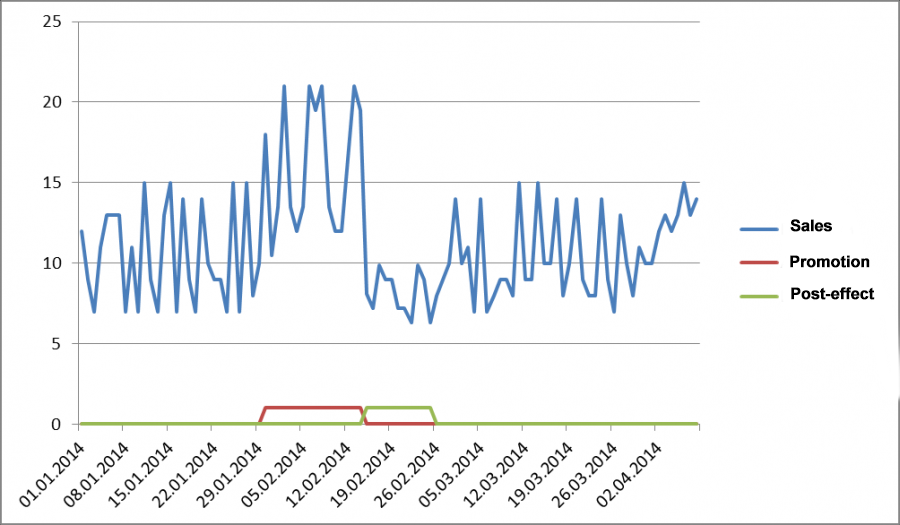
Fig 7. Sales during the marketing campaign and post-effect.
To avoid this problem, we need forecast not sales based on sales history, but demand based on demand history. To get real demand in the past period, in this case, you can apply the retrospective forecasting approach. To do this, we need to know the period of the promotion. We can get this from our account system. This is a useful thing to have at our disposal, but how do we know when and how long the post-effect occurs?
It makes sense that the post-promotion effect will depend on the jump in demand that resulted from our marketing campaign. If sales volumes doubled, then we can assume that the demand is satisfied two periods ahead. Therefore, we take the post promotion effect period as the period of the marketing campaign and forecast the demand for the period from the beginning of the campaign to the end of the post-effect.
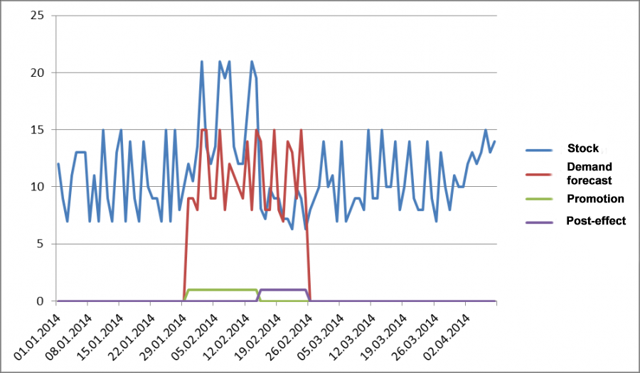
Fig 8. Forecast of Actual Demand in Prior Period.
Another way to determine the post-effect period is to estimate the forecast error in relation to the forecast error for a standard period. To do this, we build a forecast from the end of the marketing campaign to the end of the sales history. During this period, at the time of the post-effect, the forecasting error will be large, quite different from the forecasting error from pre-promotion data. At the point where the error approximates the familiar, pre-promotion error, the post-effect will disappear.
One-time large sales. Outliers and Anomalies in Demand.
We may have a client a client come and buy 10 times more in one purchase than we sell on average per day. If this is a one-time case and unusual for us, obviously, there is no need to keep stock on hand or calculate our inventory based on this case. But when we go to forecast sales, we'll end up with an exaggeratedly high inventory number without excluding such unusual buyers. Below is an example where an unusual customer bought 60 items on January 11. This is equal to our 12 day sales volume.
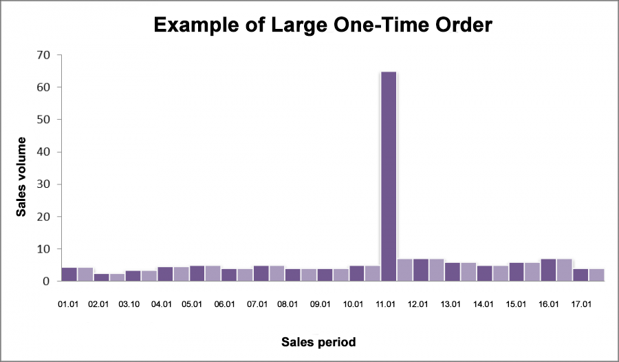
Fig 9. Example of Large One-Time Order.
If we include this outlier, the model will either pick up on a false pattern, or we will end up with a large forecasting error for this POS. In the first case, we may unexpectedly end up with overstock. In the example below, the model picked up on a false trend and repeated it in the future.
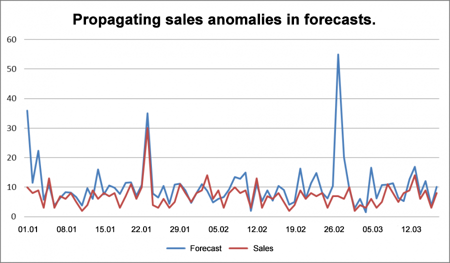
Fig 10. Propagating sales anomalies in forecasts.
In the second case, we will have a major overshot in calculating our safety stock, which depends on forecast errors or sales cycles.
Let's take a closer look at this case. For purposes of illustrating the point, we'll build our forecast based on the average. The average without this outlier is 4.8 units. Including the one-time large order, it's 8.3 units. Note that 8.3 units exceeds our maximum daily sales. Thus, if we focus on this number, we are guaranteed to order overstock even if we have forecast demand. Let's see what happens with the safety stock in this case. We may use safety stock to protect against variations in demand or forecasting errors. Using sales fluctuations in essence implies that we use the average forecast for our business.
|
|
Safety stock Without filtration |
Safety stock With filtration |
|
Service level 95% Planning horizon of 5 days |
53,8 |
4,8 |
|
Service level 98% Planning horizon of 5 days |
67,2 |
5,9 |
|
Service level 95% Planning horizon of 30 days |
131,9 |
11,7 |
|
Service level 98% Planning horizon of 30 days |
164,7 |
14,6 |
As we can see from the table, the safety stock will be 11.2 times greater if we don't omit the outlier. The most interesting thing is that with a service level of 95% and a planning horizon of 5 days, the safety stock will still be insufficient to meet demand for this type of customer.
Now, how would a one-time large order impact our overall inventory level if we ignore the order?
|
|
Total stock Without filtration |
Total stock With filtration |
Ratio |
|
Service level 95% Planning horizon of 5 days |
53,8+41,5=95,3 |
4,8+24=28,8 |
3,27 |
|
Service level 98% Planning horizon of 5 days |
67,2+41,5=108,7 |
5,9+24=29,9 |
3,63 |
|
Service level 95% Planning horizon of 30 days |
131,9+249=380,9 |
11,7+144=155,7 |
2,45 |
|
Service level 95% Planning horizon of 30 days |
164,7+249=413,7 |
14,6+144=158,6 |
2,6 |
It is easy to see that if we plan for a short period, the error caused by the outlier is much more significant than if we're planning over the long term. But even in the case of a long-term period, we have much more overstock than needed. This is therefore an effect we need to handle, by knowing how, first of all, how to identify such outliers, and then knowing how to deal with them.
How do we detect outliers?
The first thing is to remember that a sales anomaly is a somewhat rare event, and doesn't occur often. In the example below, we have two potentially anomalous sales, visible to the naked eye.
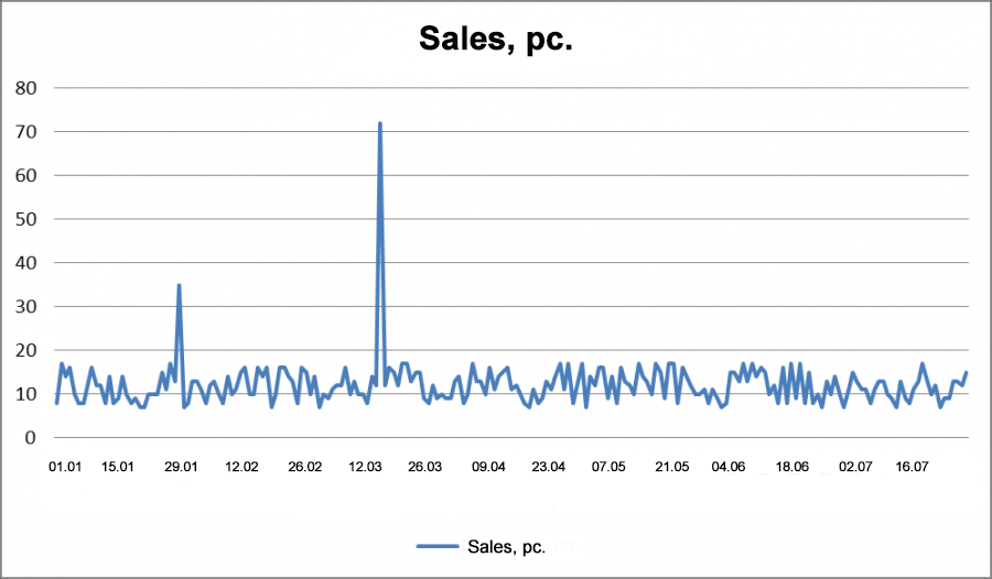
fig 11. Chart of Abnormal Sales.
In order to be sure that these are anomalies, we will calculate how many times there are sales of different volumes over the entire history and divide by the total number of days in our sales history. If we consider this number as a percentage (we multiply it by 100), then this will be the frequency of occurrence of a given sales volume over the entire history.
|
Sales volume |
Sales volume frequency |
|
7 |
5,74% |
|
8 |
12,44% |
|
9 |
7,66% |
|
10 |
13,88% |
|
11 |
7,66% |
|
12 |
8,61% |
|
13 |
11,48% |
|
14 |
8,13% |
|
15 |
6,70% |
|
16 |
8,61% |
|
17 |
8,13% |
|
35 |
0,48% |
|
72 |
0,48% |
|
Total |
100,00% |
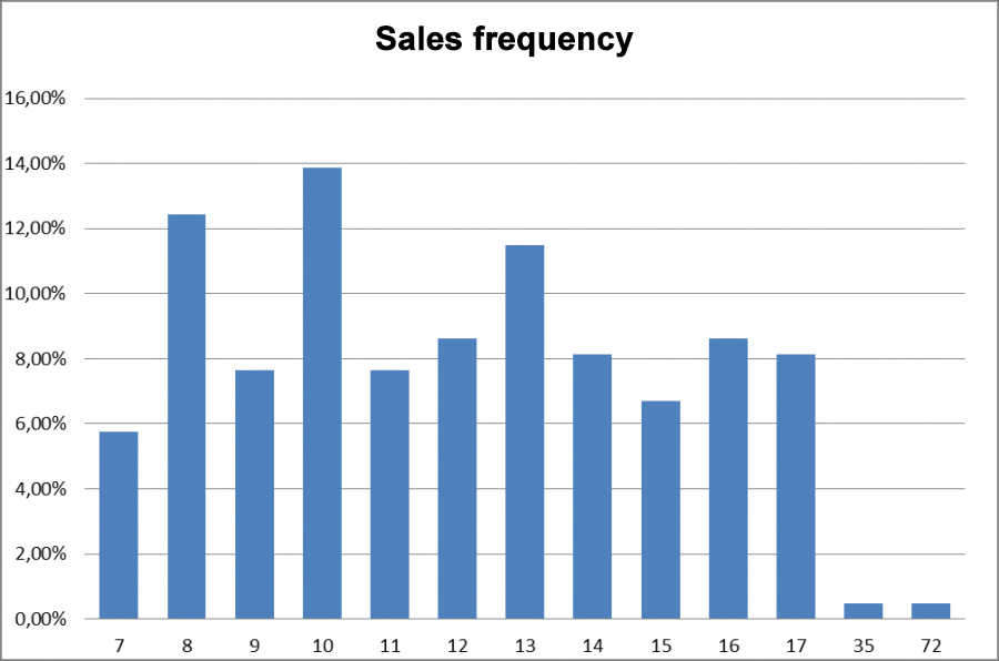
Fig 12. Sales frequency.
Outliers are abnormally large sales that we do not want to take into account when forecasting. But we need to recognize where an exceptional sale is a normal situation for our business and plan accordingly. We must take into account for example the spike in demand for flowers on March 8, Women's Day, when planning in the future and cannot simply exclude it from the history of sales. On the other hand, the fact that an event is rare or exceptional does not automatically mean that it is an outlier. If medium sales are rare, that's no biggie. It would seem that we can just sort by sales volume and exclude those frequencies from the tails that are less than a certain threshold, for example, 1%. Then we successfully filter out sales of 35 and 72 units. But what happens if our demand is too variable and the same sales volumes rarely repeat?
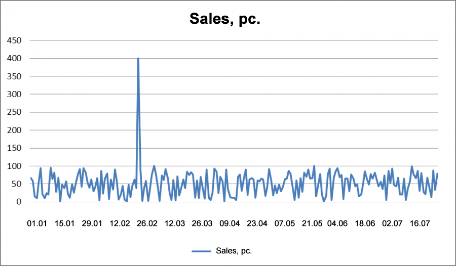
Fig 13. Sales with Outlier.
Take a look at the chart with the frequency of sales. If we filter at 2%, then we'd include all sales from 100 to 91 units, which would be a mistake. In this case we could end up excluding the entire sales history if it was extremely variable.
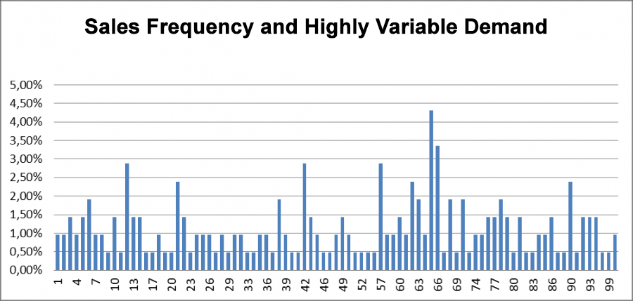
Fig 14. Sales Frequency and Highly Variable Demand.
To prevent this error, we can use a threshold value for the aggregate rather than specific frequencies, similar to what is done when using ABC group segmentation.
|
Number |
Sales frequency |
Cumulative amount of sales frequency |
|
1 |
0,96% |
0,96% |
|
2 |
0,96% |
1,91% |
|
3 |
1,44% |
3,35% |
|
4 |
0,96% |
4,31% |
|
5 |
1,44% |
5,74% |
|
6 |
1,91% |
7,66% |
|
7 |
0,96% |
8,61% |
|
8 |
0,96% |
9,57% |
|
9 |
0,48% |
10,05% |
|
10 |
1,44% |
11,48% |
|
... |
... |
... |
|
87 |
0,48% |
89,95% |
|
88 |
0,48% |
90,43% |
|
90 |
2,39% |
92,82% |
|
91 |
0,48% |
93,30% |
|
92 |
1,44% |
94,74% |
|
93 |
1,44% |
96,17% |
|
94 |
1,44% |
97,61% |
|
96 |
0,48% |
98,09% |
|
99 |
0,48% |
98,56% |
|
100 |
0,96% |
99,52% |
|
400 |
0,48% |
100,00% |
|
Total |
100,00% |
Let's use a threshold (tolerance) of 1.0%. Then the aggregate frequency should not exceed (100 - 1.0%) = 99.0%. Anything that has a cumulative probability of more than 99.0% is labeled as a potential outlier. Could we get lost in the statistics in a case like this? Fortunately, we can’t, since in the worst case scenario we will lose 1% of the entire history, with a history of 300 days, we will flag only 3 dales, even if the sales are different.
What do we do with the sales anomalies we've found?
The sales anomalies are data points in the historical data, and not entire periods like we are dealing with in the case of out-of-stocks. Therefore we can replace the updated data to use for the median or mean calculated without the outliers. The median in our case will be the volume of sales where the aggregate probability is 50%. In our example, this is 56 units, and the average is 49 units. This is a pessimistic approach; it assumes that there were no other higher than average sales other than anomalies. It ignores the possibility that on that day there could have simply been large sales from a client who decided to make an unusually large order. We are excluding not only this particular customer, but a large order. Of course, you could just look at specific sales slips and POs and exclude them. But then a situation may arise where unusually high sales are not associated with a specific client, but with other events. In this case, abnormal sales on the day we're looking at are caused by a number of factors, and a large number of clients together were responsible for the unusually high sales number. If we look at individual order receipts and PO's we will fail to notice this.
As an optimistic substitute, we could replace abnormally high sales with the highest sales that remain after the exclusion of sales anomalies. In our example, this would be 99 units. This gives us the following snapshot of past sales:

Fig 15. Sales After Excluding Outliers.
We have eliminated the effect of external events on demand in the past, but we must keep in mind that forecasting must account for expected future events, such as sales ad campaigns, holidays or sales promotions.
We know that we need to forecast demand based on historical demand. Trying to forecast demand based on sales history will be of little benefit. Just as it would be to try to forecast sales based on demand history. But does it always make sense to forecast demand? The ultimate goal here is to determine the optimal inventory level we need to meet demand at a given service level. Sometimes the forecast error is so high that it makes no sense to make a forecast. Could we just skip this and calculate the optimal inventory level? We actually can, in fact.
Part II. Can you - and should you - always forecast demand?
What do your sales look like? Not the top selling items, but the majority that you want to forecast for? Do they happen daily or once a week or maybe monthly? This will determine whether or not you can actually forecast demand. If we can't forecast demand, what tool will help us optimize our inventory?

Fig 16. Sales with Regular, Even Demand
Sales aren't always as regular and even as the above graph. This is especially true of trade in auto parts, electrical goods, building materials, office supplies, household chemicals, thermal equipment and other goods. That is, almost everything except food and beverages. Demand for these products is quite flat. It happens - or it doesn't. How do we identify intermittent demand? We calculate the average interval between sales. If we have two sales in a row, the interval is 1 day. If we had instead a sale on one day, and then no sales for two days, and then had an order on the third day, our interval would be three days. We can use these intervals to find an average value. If the average value, the so-called ADI (average inter demand interval)> 1.25, then demand is intermittent. Empirical evidence shows that there is little benefit in using classical forecasting methods like exponential smoothing, the Hold-Winters method, ARIMA, and other single point forecasts on such data.
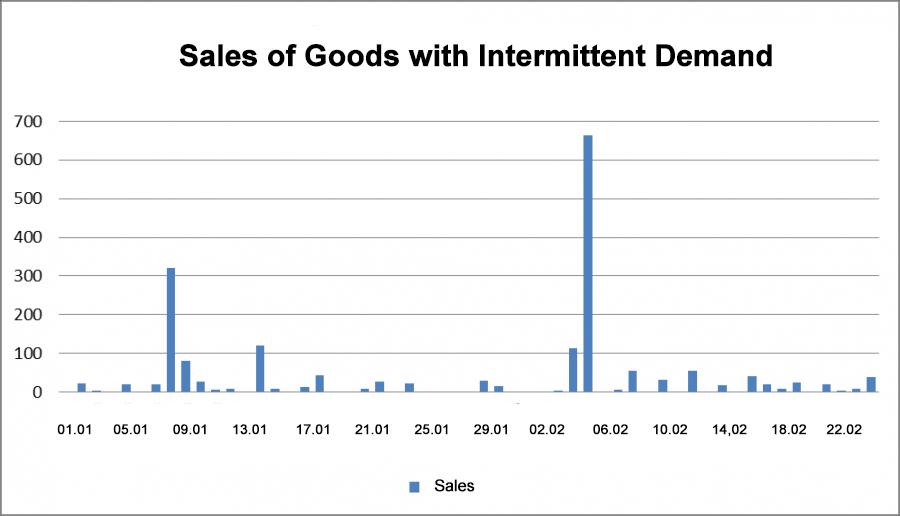
Fig 17. Sales of Goods with Intermittent Demand.
What can we do?
There are two options. The first is to try to group our data to minimize the average intervals between sales. We move from planning daily to weekly/monthly planning while grouping the sales history by week/month. This option will not always work. If we need to know inventory for one to two days, then grouping by weeks - or months - won't give us insight on this specific question. This grouping or bucketing will also introduce an artificial dependence between the data and reduce the variability of demand, which would be a mistake.
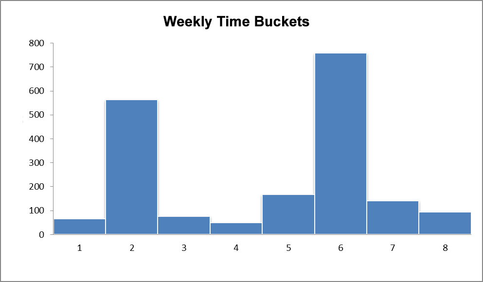
Fig 18. Weekly Time Buckets.
The second option is to use probabilistic forecasting methods. Probabilistic forecasting models, such as Efron, Dekker, and Willemaine have been shown effective in forecasting slow (intermittent) demand.
Using Probabilistic Models
It was previously believed that Z group items were not forecastable due to their highly variable and unpredictable demand. Expert ad hoc reviews were usually used. And the complexity of the task and the errors are not surprising - it’s the same as trying to hit a target that moves erratically and changes in size from day to day. In contrast, probabilistic methods are like using a whole team of shooters who will hit the target at a certain level of accuracy; these methods make it possible to manage an entire product range rather than just using items with smooth demand.
If you look at the assortment of goods in general, it turns out that very few goods have smooth demand. Take food and beverage for example, which is considered to have smooth demand. But even for this segment, only 6% of 50 000 SKUs show stable demand. The other 47 000 items have intermittent demand. For other product categories, such as auto parts, building materials, electrical goods, plumbing, etc, we will have 98-99% of all SKUs with intermittent demand.
Classical methods won't work well at all here. By 2008 they were already proven to be ineffective. Probabilistic algorithms have advanced far past the classic models and help eliminate the human factor in product range management.
Key Advantages Over Classic Models
All classical forecasting algorithms work according to one scenario. You input your sales history and end up with a demand forecast in the form of a single point, and then add your safety stock to that number. When calculating the forecast safety stock for each item, some standard distribution is used: normal or, for example, Poisson. In fact, this distribution is not characteristic of grocery and food products in 96% of cases and a poor fit in 99% of cases for other areas of trade and distribution.
When we use a probabilistic model, we get a range of probabilities. For example, we can find that the probability of selling 10 units a day is 15%, and we can sell 15 items with a 22% probability. And if we want to cover 95% of cases of potential demand (to provide a first-class service level of 95%), then we need to have 22 items on hand. It’s like a weather forecast. You're not going to be too happy if you're told tomorrow will be sunny and end up caught in the rain without an umbrella. But if you are warned there is a 30% chance of rain, you will be able to be prepared. This way, we can determine the target service level in advance and purchase exactly as many goods as we need.
It is worth nothing that service level is also a probability. And some buyers who order safety stock based on a service level believe that they are using probabilistic models. This is quite mistaken however. It is helpful to understand that our system output is a single data point as a forecast of sales and a confidence interval or set of sales levels with differing probabilities.
The below example is an inventory calculation for spark plugs.
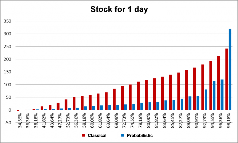
Fig 19. Sample inventory calculation for spark plugs for 1 day.
The X axis shows service level; the Y axis is the required inventory.
As you can see from the graph, we end up with overstocks when using classic forecasting and a low service level. Moreover, our inventory on hand is 4 times greater in some cases compared to probabilistic models. When planning for a longer period, the same trend is observed.
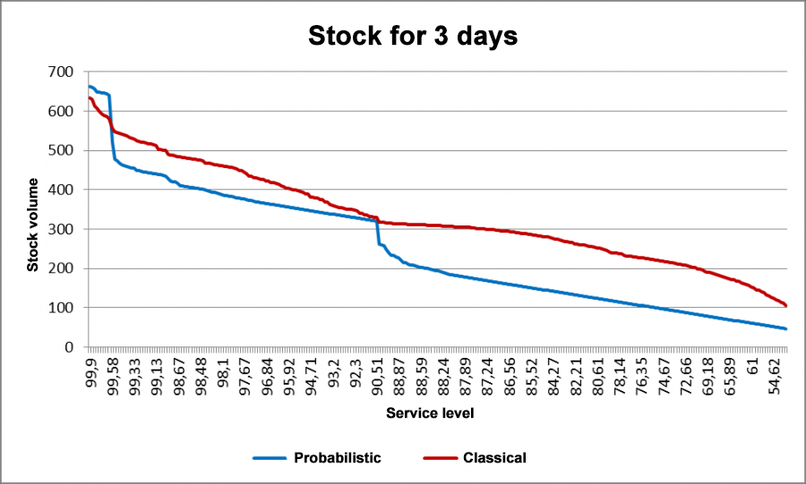
Fig 20. Sample inventory calculation for spark plugs for 3 days.

Fig 21. Sample inventory calculation for spark plugs for 7 days.
Service Level Management
Is it possible to set a service level for each item and try to achieve it? While this is possible, this model fell out of use already in 2012.
Various losses (from stock-outs, holding costs, delays, etc.) also have a probabilistic distribution and to minimize the total losses, we need to optimize the service level for each order!
Unlike classic forecasting methods, probabilistic models allow you to control the service level and minimize total losses on the fly. Companies can independently (or automatically, using specialized software) calculate the optimal level of service for each product. This will help reduce risks in cases where the sale of an additional quantity of goods does not cover the holding or shipping costs.
Today probabilistic methods are considered to be one of the most accurate approaches for inventory management and have shown their superiority over classic models. In Western countries, these methods are applied de facto and have long replaced older models. In Russia, this standard is only beginning to gain momentum, but nevertheless, many companies have already begun to appreciate its advantages.
Scientific background. Poor Fit of Classic Forecasting Models for Intermittent Demand.
One of the first methods used to forecast demand based on time series is the method of exponential smoothing [1]. This method can be used to forecast uniform demand.
In 1972, Croston[2] showed that exponential smoothing is a poor tool for forecasting intermittent demand, and proposed his own model, in which intervals between purchases and their volumes are separately forecasted.
A 2001 article[3] showed that the Croston method features bias and proposed an improvement on the model
The method of exponential smoothing is based on the assumption that the time series is stationary. If there is a trend, it needs to be extrapolated. Holt's linear method[4] relies on an estimate of the local average value and growth rate.
Another option for handling trends is the use of a moving average. In this case, the forecast is not based on the entire volume of historical data, but using only the most recent part of the data.
One of the most common options for integrating the moving average, exponential smoothing, linear trend and random walk is the ARIMA model.
These models were created as part of a parametric approach to modeling random processes. They assume that sales (and the intervals between them in the Croston model and variations on it) have a known distribution. Many variations of these models have been developed, based on the use of various classical distributions. Empirical data show that intermittent demand is poorly captured using classic distributions.
The practical application of such models requires an analysis of distributions in an expert manner in each specific situation and may not give a satisfactory result.
References
|
[1] ↑ |
R. J. Hyndman, A. B. Koehler, J. K. Ord и R. D. Snyder, Forecasting with Exponential Smoothing: The State Space Approach, Berlin: Springer, 2008. |
|
[2] ↑ |
J. D. Croston, «Forecasting and stock control for intermittent demands,» Operational Research Quarterly, № 23, p. |
|
[3] ↑ |
A. A. Syntetos и J. E. Boylan, «On the bias of intermittent demand estimates,» International Journal of Production Economics, № 71, p. |
|
[4] ↑ |
C. C. Holt, «Forecasting seasonals and trends by exponentially weighted moving averages,» International Journal of Forecast, № 20, p. |
|
[5] |
A. A. Syntetos и J. E. Boylan, «The accuracy of intermittent demand estimates,» International Journal of Forecasting, № 21, pp. |
|
[6] |
R. D. Snyder, «Forecasting sales of slow and fast moving inventories,» № 140, pp. |
|
[7] |
L. Shenstone и R. J. Hyndman, «Stochastic models underlying Croston’s method for intermittent demand forecasting,» Journal of Forecasting, pp. |